Model > Evaluate > Evaluate classification
Evaluate model performance for (binary) classification
To download the table as a csv-files click the download button on the top-right of your screen. To download plots as png files click the download icon on the middle-right of your screen.
Response variable
Select the outcome, or response, variable of interest. This should be a binary variable, either a factor or an integer with two value (i.e., 0 and 1).
Choose level
The level in the response variable that is considered a success. For example, purchase or buyer is equal to “yes”.
Predictor
Select one or more variables that can be used to predict the chosen level in the response variable. This could be a variable, an RFM index, or predicted values from a model (e.g., from a logistic regression estimated using Model > Logistic regression (GLM) or a Neural Network estimated using Model > Neural Network (ANN)).
# quantiles
The number of bins to create.
Margin & Cost
To use the Profit and ROME (Return on Marketing Expenditures) charts, enter the Margin for each sale and the estimated Cost per contact (e.g., mailing costs or opportunity cost of email or text). For example, if the margin on a sale is $10 (excluding the contact cost) and the contact cost is $1 enter 10 and 1 in the Margin and Cost input windows.
Show results for
If a filter is active (e.g., set in the Data > View tab) generate results for All data, Training data, Validation data, or Both training and validation data. If no filter is active calculations are applied to all data.
Plots
Generate Lift, Gains, Profit, and/or ROME charts. The profit chart displays a profit index useful to compare performance across predictors/models
Example
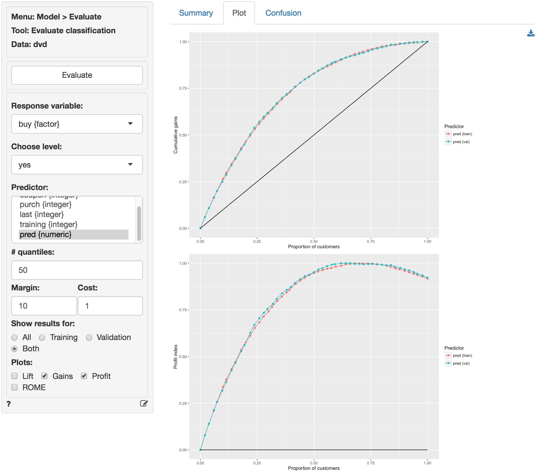
The Gains and Profit charts below show little evidence of overfitting and suggest that targeting approximately 65% of customers would maximize profits.
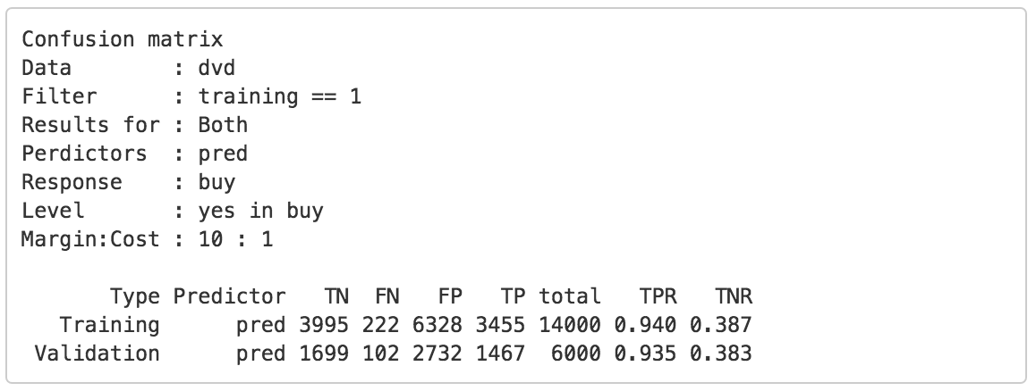
This insight is confirmed by looking at the confusion matrix. The True Positive Rate in the training and validation sample are 94.0% and 93.4% respectively.
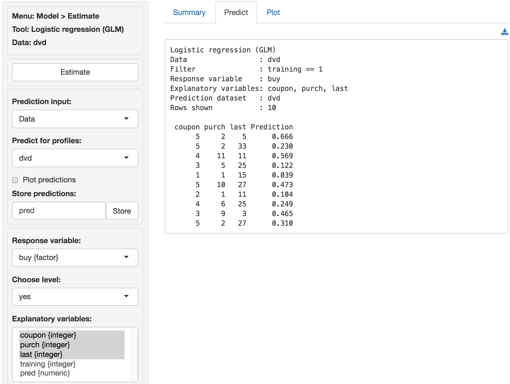
The prediction used in the screen shots above was derived from a logistic regression on the dvd data. The data is available through the Data > Manage tab (i.e., choose Examples from the Load data of type drop-down and press Load examples). The model was estimated using Model > Logistic regression (GLM). The predictions shown below were generated in the Predict tab.